User guide

Introduction

What is grempy?

grempy (GRanada ElectroMagnetic PYthon simulator) is a pure Python Finite-Differences Time-Domain (FDTD) electromagnetic solver. Its main purpose is the study of the interactions between a lightning-generated electromagnetic pulse (EMP) and the upper layers of planetary atmospheres.

The code was developed by Alejandro Luque at the Instituto de Astrofísica de Andalucía (IAA), CSIC and is released under the GPLv2 license.

Although many good and open source general-purpose FDTD codes are available, such as MIT’s Meep, grempy has the more restricted purpose of simulating the propagation of the EMP generated by a lightning stroke and its interaction with the lower ionosphere. This process is the responsible of so-called ELVEs (Emissions of Light and Very low frequency perturbations due to Electromagnetic pulse sources). Elves are expanding, ring-shaped light emissions located at about 100 km altitude, centered above the originating lightning and lasting less than or about 1 ms. Restricting its domain, grempy is easier to use than general-purpose FDTD solvers.

Some features of grempy are:

• Self-consistently solves the Langevin (or modified Ohm equation) with an altitude-dependent mobility.
• Incorporates non-linear processes such as local changes in the ambient conductivity due to impact-ionization.
• The properties of the atmosphere where the EMP propagates are easily specified with text files that specify the altitude profiles of background gas density and initial electron density. The nonlinear response of the electron density is also specified by an external file. See section Defining an atmosphere
• A plug-in system permits the extension of the code with simple Python modules. This can be used, for example, to simulate additional chemical processes.

Installation

Required Python libraries

grempy uses some Python libraries for the numerical computations as well as its output format and plotting. You have to have them installed and accesible to run grempy:

• NumPy and SciPy. See here for installation instructions for your operating system.
• Matplotlib
• h5py
• pyYAML

For Linux and Mac OS X we recommend using the package repositories of your distribution or MacPorts/Homebrew for Macs.

Installation

You can fetch the latest version of grempy from github using:

git clone https://github.com/aluque/grempy.git

This will download the required files into your current folder. Since grempy is written 100% in python, you do not need any additional compilation or instalation.

Running a simulation

Once the code is set up, you use the script em.py to start a simulation:

python /path/to/em.py simulation.yaml

where the file simulation.yaml contains the input parameters of the simulation. See Input parameters for a list of all valid parameters with a short description.

Input files

Input files for the code are .yaml files with key/value pairs. The YAML format is a light-weight serialization format. You can obtain more information about this format at yaml.org.

grempy expects an input file formed by key/value pairs specified as:

key: value

Here is an of an input file for grempy:

#
#  FILES AND DIRECTORIES
#
#  The directory that contains extra input files.
input_dir: /your/input/folder/earth/

#  A file to read the gas density from in h[km] n[cm^3].
gas_density_file: gas.dat

#  A file to read the electron density from in h[km] n[cm^3].
electron_density_file: electrons.dat

#  File with the ionization rate
ionization_rate_file: ionization.dat


#
#  SIMULATION DOMAIN
#
#  Radius of the simulation domain in km.
r: 400.0

#  Lower boundary of the simulation in km.
z0: 0.0

#  Upper boundary of the simulation in km.
z1: 110.0

#  Number of cells in the r direction.
r_cells: 400

#  Number of cells in the z direction.
z_cells: 110

#
#  TIMES
#
#  The time step in seconds.
dt: 1e-07

#  The final simulation time.
end_t: 0.050

#  The time between savings in seconds.
output_dt: 1e-04

#
#  CURRENT SOURCE
#
#  The Charge transferred in C.
Q: 150.0

#  With of the source in km.
r_source: 1.0

#  Lower edge of the source in km.
z0_source: 0.0

#  Upper edge of the source in km.
z1_source: 10.0

#  Rise time of the stroke in seconds
tau_r: 1e-3

#  Fall (decay) time of the stroke in seconds
tau_f: 2e-3


#
#  GAS PROPERTIES
#
#  Mobility times N in SI units.
mu_N: 1.2e+24


#
#  BOUNDARY CONDITIONS
#
#  Number of cells in the convoluted perfectly matching layers.
ncpml: 10

# Lower boundary condition.  Use 0 for a cpml, != 0 for an electrode
lower_boundary: 1

#
#  TRACKING OF THE FIELDS AT SOME POINTS
#
track_r: [40, 50, 60, 80, 100]
track_z: [50, 51, 52, 53, 54, 55, 56, 57, 58, 59,
          60, 61, 62, 63, 64, 65, 66, 67, 68, 69,
          70, 71, 72, 73, 74, 75, 76, 77, 78, 79,
          80, 81, 82, 83, 84, 85, 86, 87, 88, 89]

Defining an atmosphere

grempy makes it easy to specify the properties and initial state of the atmosphere where the EMP is propagating. The input parameter input_dir helps the user to organize different input conditions into separate folders. All filenames are relative to the folder indicated by input_dir. In the distributed code we include samples of three planetary atmospheres: for Earth, Jupiter and Saturn.

The profile of background gas density as a function of altitude is read from the file specified in the parameter gas_density_file. The file must contain two columns, the first one is altitude in kilometers; the second is the gas density in cm^-3.

An additional file provides the initial electron density as a function of altitude. The name of this file is read from the parameter electron_density_file. The format is the same as above: two columns, the first one is altitude in kilometers; the second is the electron density in cm^-3.

The background gas composition influences the propagation of electromagnetic waves first by setting the electron mobility and second by setting a rate of ionization as a function of reduced electric field. The mobility is specified in the parameter mu_N. This must give, in SI units, the electron mobility \(\mu\) times the background gas density \(n\). The product of the two is assumed to be constant.

The ionization rate is read from the file specified in the parameter ionization_rate_file, that must contain two columns: a reduced electric field \(E/n\) in Townsend (1 Td = 10¹⁷ V cm²). and an ionization rate in m³/s.

Output files

The code produces a single output file per simulation. The name of the output file is constructed by replacing .yaml for .h5 in the input file name. The output is a HDF5 file, organized as follows:

The root group of the HDF5 file contains attributes containing the input parameters used in the simulation as well as information about the running environment encoded into atributes that start and end with underlines:

_command_

The command that was used to start the simulation.

_timestamp_

The machine time when the simulation was started.

_ctime_

Human-readable version of _timestamp_.

_cwd_

The current directory when the program was run.

_user_

Login name of the user that run the simulation.

_host_

The name of the computer where the simulation run,

In the root group we also store this information for efficiency reasons:

box

An array specifying the simulation domain (r0, r1, z0, z1).

dim

An array containing the number of cells in the r- and z-directions.

ngas

An array with the gas density depending on the altitude.

Each time-step is saved as a sub-group of a steps group, with names 00000, 00001 and so forth. For every step we save the following data, all of it using SI units.

te (attribute)

The time at which the electric field is saved.

th (attribute)

The time at which the magnetic field is saved.

timestamp (attribute)

Machine time when the snapshot was saved.

er, ez, ephi (datasets)

The components of the electric field, stored as 2d arrays (r-index, z-index).

hr, hz, hphi (datasets)

The components of the magnetic field, stored as 2d arrays (r-index, z-index).

ne (dataset)

The density of free electrons, also as a 2d array.

j (dataset)

The current density, also as a 2d array.

Besides, each snapshot contains also information about the status of the CPML included in the simulation. They are stored as sub-groups of each timestep with names cpml_000, cpml_001, ...

Plotting

The script plotter.py can be used to plot the results of a simulation for a quick inspection. Use it as:

usage: python plotter.py [-h] [-o OUTPUT] [-d OUTDIR] [--list] [--parameters]
                         [--log] [--show] [--zlim ZLIM] [--rlim RLIM]
                         [--clim CLIM] [--cmap CMAP]
                         [--figsize FIGSIZE FIGSIZE] [--vars]
                         input [var] [step]

Positional arguments:

input	HDF5 input file
var	Variable to plot
step	Step to plot (‘all’ and ‘latest’ accepted)

Options:

-o={rid}_{step}_{var}.png, --output={rid}_{step}_{var}.png
	Output file (may contain {rid} {step} and {var})
-d={rid}, --outdir={rid}
	Output directory (may contain {rid} and {var})
--list=False, -l=False
	List all the simulation steps
--parameters=False, -p=False
	Show the simulation parameters
--log=False	Logarithmic time scale
--show=False	Interactively show the figure
--zlim	Limits of the z scale (z0:z1)
--rlim	Limits of the r scale (r0:r1)
--clim	Limits of the color scale (c0:c1)
--cmap=invhot	Use a dynamic colormap
--figsize=[12, 6]
	width height of the figure
--vars=False	Print a list available variables to plot

Sub-commands:

In the above, {rid} refers to the run identifier, which is the input filename stripped of the .h5 extension, {step} refers to the plotted step (e.g. 0013) and {var} to the plotted variable.

Some of the possible variables to plot are:

eabs

Absolute value of the electric field.

en

Reduced Field \(E/n\).

er

z component of the electric field.

ez

z component of the electric field.

ne

Electron density.

jr

r component of the current density.

jz

z component of the current density.

photons

Integrated photon emissions (if available)

energy

Deposited energy density [$mathdefault{J m^{-3}}$]

max_eabs

Highest electric field at each point

max_en

Highest Reduced Field \(E/n\) at each point.

If –show is given, the program will open a matplotlib window; otherwise a .png file will be saved as specified by --output and --outdir.

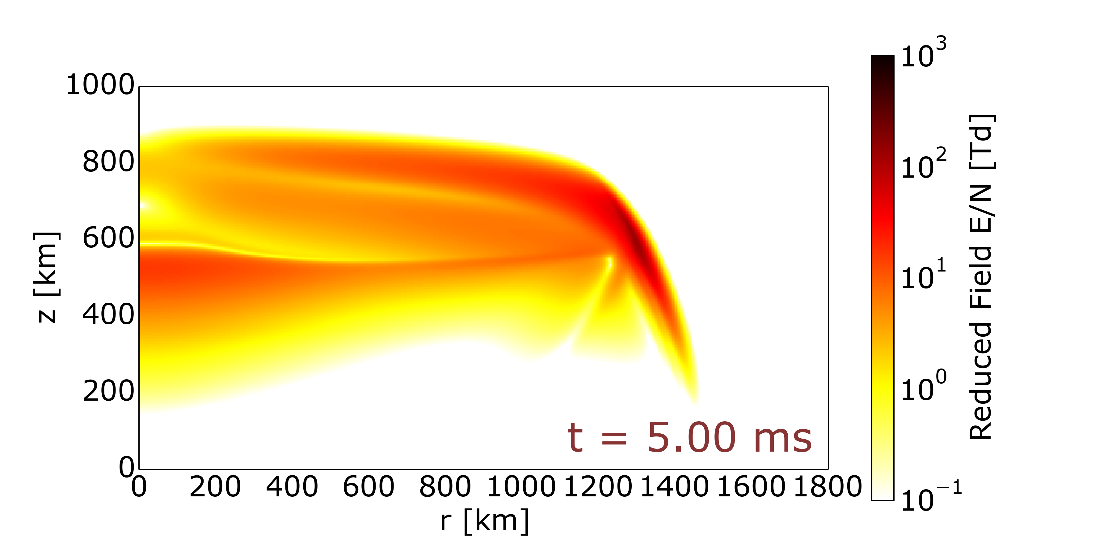
For example, tlot the reduced electric field at step 0010 of a simulation file output.h5, plotting r from 0 to 1800 km and z from 0 to 1000 km, using a logarithmic colorscale from 10^-1 to 10³ Td use:

python plotter.py output.h5 en 0010 --log --rlim=0:1800 --zlim=0:1000 --clim=1e-1:1e3

That produces the following output: