2. PANIC Quick-Look Tool (PQL)
2.1. Purpose
PANIC Quick-Look (hereafter PQL) performs some on-line data processing for quick-look or quality check of the data being acquired, taking a close look at a raw near-infrared image and getting a quick feedback of the running observation.
PQL is an application with a graphical user interface which monitors the GEIRS data output, waiting for new FITS files coming from GEIRS. When a new file is detected, it is added to the file list view in the main panel, and then PQL will perform the task previously specified by the user in the setup configuration. Some of the available tasks are:
Only display the FITS image with no processing
Dark subtraction, flat division
Sky subtraction (using N-nearest frames or own sky )
Field distortion removal
Image align and stacking
Preliminary astrometric solution
Preliminary photometry
In addition, PQL allows you to execute manually in an interactive way some tasks with the data. For example, you will be able to select a file, compute some statistics values (background, FWHM, min, max, …) or ask for the sky subtraction looking for the nearest N frames around the selected one. Other option available is to select a set of files and request to shift and align them.
PQL can be operated in both near-real time mode (during the observation) and offline mode (after the observation, with all data files already stored in the disk); however, its functionalities have been provided mainly in near-real time to check the status and progress of the observation during the night.
The visualization application used to display the images is SAOImage ds9, which supports FITS images, multiple frame buffers, region manipulation, and many scale algorithms and colormaps.
2.2. FITS files and headers
PQL only supports FITS (Flexible Image Transport System) with two-dimensional
image formats. Because PANIC has a FPA of four detector, the FITS files can be Single Extension FITS (SEF)
or Multi-Extension FITS (MEF), however MEF are prefered.
The complete definition of the FITS headers can be found on the GEIRS documentation.
For general purpose, such as viewing and simple analysis, only minimal headers keywords are required. However, and in order to group and reduce observing sequences, the following header keywords are also required:
OBS_TOOL= 'OT_V1.1 '           / PANIC Observing Tool Software version
PROG_ID = '        '           / PANIC Observing Program ID
OB_ID   = '6       '           / PANIC Observing Block ID
OB_NAME = 'OB CU Cnc Ks 2'     / PANIC Observing Block Name
OB_PAT  = '5-point '           / PANIC Observing Block Pattern Type
PAT_NAME= 'OS Ks 2 '           / PANIC Observing Secuence Pattern Name
PAT_EXPN=                    1 / PANIC Pattern exposition number
PAT_NEXP=                    5 / PANIC Pattern total number of expositions
IMAGETYP= 'SCIENCE '           / PANIC Image type
These keywords are automatically added to the FITS header by the PANIC Observation Tool, as each file is created. If these are not saved, PQL will not work correctly.
2.3. Starting PQL
To start PQL GUI, you can lauch it from the PANIC computer (panic22/panic35) once you are logged as obs22/obs35 user. Thus, as any one of the workstations of the observing room, open a X terminal window and log into the PANIC computer as follow:
for 2.2m:
$ ssh -X obs22@panic22
(ask Calar Alto staff for password)
for 3.5m:
$ ssh -X obs35@panic35
(ask Calar Alto staff for password)
Once you are logged into the PANIC computer, to launch PQL GUI type next command:
$ start_ql &
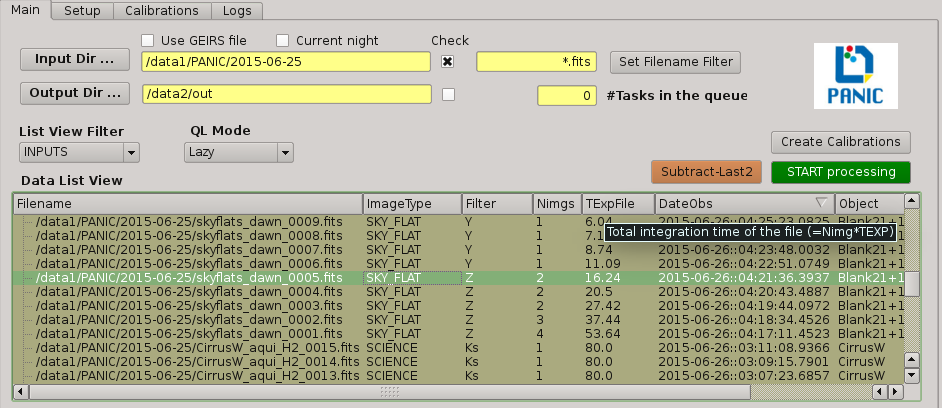
The next figure shows a snapshot of the main window of PQL GUI that will bring up the start_ql command.

2.4. Configuration files
The configuration files used by PQL are located in the $PAPI_HOME/config_files. The main config file is the same file used by PAPI, ie., $PAPI_CONFIG, and usually called papi.cfg.
This file includes a lot of parameters used by PAPI, and therefore by PQL during the processing; however at the end of the $PAPI_CONFIG file there is section called quicklook, where the user can set some specific parameters for PQL:
##############################################################################
[quicklook]
##############################################################################
# Next are some configurable options for the PANIC Quick Look tool
#
# some important directories
#
source = /data1/PANIC/
output_dir = /data2/out   # the directory to which the resulting images will be saved.
temp_dir = /data2/tmp    # the directory to which temporal results will be saved
verbose = True

# Run parameters
run_mode = Lazy # default (initial) run mode of the QL; it can be (None, Lazy, Prereduce)
Although the user can edit these values in the config file, some of them can be set easily on PQL’s GUI.
For the complete list of the parameters available on the $PAPI_CONFIG file, see Main config file section.
2.5. PQL’s main window
PQL Main window contains a Menu bar (1), Tool bar (2), four Tabbed panels (3) and an Event Log Window (4). Images are displayed in an external well-known application, ds9. Plots results are displayed in the additional windows, usually generated by matplotlib than can be copied to the clipboard, printed or saved.
2.5.2. Tool bar
The tool bar duplicates some of the options available from the menu bar or the pop-up menu. Currently, there are several buttons which provide quick access to change the most frecuently-used PQL actions:
add a file to the current view
change the source input directory: the same that Input directory.
display the current selected image: the same that Display.
open an IRAF console
open Aladin tool
quit PQL (on the right border)

2.5.3. Main panel
This tab panel contains the following controls:
Input directory
Ouput directory
Filename filter
Current night
Use GEIRS file
Data list view
List view filter
QL mode
‘Subract last-2’ button
‘START processing’ button
‘Create Calibrations’ button
2.5.3.1. Data directories
In the ‘Main’ tab panel of PQL main window, the fitst thing to set up are the data directories:
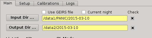
2.5.3.2. Input directory
This is where you tell PQL where the data are or being saved by GEIRS. This directory is specified at the beggining of the night on the Observation Tool. PQL requieres all data to lie in some main directory, not being required to distribute the files in individual sub-directories for darks, flats, and science images. It is advised that this directory follow the next format:
/data1/PANIC/YYYYMMDD
To set the value, the user must push the ‘Input Dir’ button:
Note that the value in this field has only effect when the checkbox on the right is clicked.
2.5.3.3. Output directory
This is where you tell PQL where the data generated by PQL, as result of some processing, will be saved. This directory must also be specified at the begining of the night, and is advised to follow the next format:
/data2/out/YYYYMMDD
To set the value, the user must push the ‘Output Dir’ button:
Note that the value in this field has only effect when the checkbox on the right is clicked.
2.5.3.4. Temporal directory
This is where you tell PQL where the temporal files generated by PQL, as result of some processing, will be saved, and probably deleted after at the end of that processing. This directory must also be specified at the begining of the night, and is advised to follow the next format:
/data2/tmp/YYYYMMDD
To set the value, the user must push the ‘Temporary Dir’ button than appears on the ‘Setup’ tab, instead the ‘Main’ tab used for input and output directory.
2.5.4. Current night checkbox
When you click this checkbox, the Input directory and Output directory fields will be automatically filled with the currect night date. If the current night Input/Ouput directories donot exist, PQL will ask you if you want to create them.
The currect night is supposed to start at 8 am (UTC) and to end at 8 am (UTC) of next day.
2.5.5. Use GEIRS file
When this checkbox is clicked, PQL will use the ~/tmp/fitsGeirsWritten file to detect the new files created by GEIRS. Files older than 1 day, will no be considered.
This detection method for FITS files is not frecuently used, but can be useful whether some problem arise reading files just after they have been written by GEIRS.
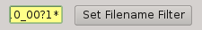
2.5.6. Filename filter
In this box, the user can filter the name of the files should appears on the data list view from the input directory (output files are not filtered). The filter can contains ‘*’ and ‘?’ wildcards.
For example:
*March10_00?1*
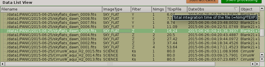
2.5.7. Data list view
Tha data list view control displays all the files found in the input directory, or in the output directory if the check box at the right of output directory is checked. Additionaly, the use can add any other FITS file. The control is a multicolum table with the next fields:
- Filename
Full path name of the file found in the
- Image type
The type of the FITS file detected: DARK, DOME_FLAT, SKY_FLAT, FOCUS, SCIENCE
- Nimgs
Number of images (layers) of the cube; if image is integrated (no cube), then = 1.
- TExpFile
Total Exposition time of the file (= Nimgs * EXPTIME) (Thus, EXPTIME = TExpFile / Nimgs)
- Date-Obs
Observation data of the file (DATE-OBS keyword)
- Object
Object name (OBJECT keyword)
- RA
Right ascention of center of the image.
- Dec
Declination of the cener of the image.
You can sort the list by any column (filename, image type, exptime, filter, date-obs, object, right ascension, declination) by clicking on their headers, as usual; by default, the list is sorted by the Date-Obs field, showing the most recect file at the top.
A double-click on any row displays all its file into SAOImage ds9.
For further details of any of the files, you can also look at the header of a fits image using ds9 using the “File/Display Fits Header…” menu option.
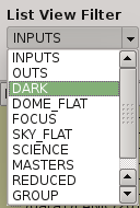
2.5.8. List view filter
It allows you to select the type of files to be shown in the data list view. The options are:
- INPUTS
Files of the input directory
- OUTS
Files of the ouput directory
- DARK
Files marked (IMAGETYP) as DARK images
- DOME_FLAT
Files marked as DOME_FLAT image
- FOUCS
Files marked as FOCUS image from a focus series
- SKY_FLAT
Files marked as SKY_FLAT images
- SCIENCE
Files marked as SCIENCE image or with unknown type.
- MASTERS
Files marked as MASTER calibration files produced by PAPI
- REDUCED
Files marked as calibrated by PAPI
- GROUP
Special case that show all the files groupped as observed sequences (OBs)
- ALL
Show all the files, not matter the type of it
2.5.9. QuickLook mode
The quick look mode combo box allows you to select the mode in which PQL will be run when the START processing button is pushed. The current modes are:
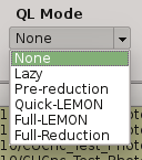
- None
No processing action is done
- Lazy (default)
If the end of a calibration (DARK, FLAT) sequence is detected, the master file is built. Otherwise, the SCIENCE files are processed as specified in the ‘Setup->Lazy Mode’:
Apply DARK + FLAT + BPM
Subtract Last Frame (Science)
Subract Nearest Sky
- Pre-Reduction
If the end of observing sequence is detected, it is processed in a quick mode (single pass for sky subtraction). For calibration sequences, the master file will be built, and for science sequences, a quick reduction will be done using options configured in the ‘Setup->Pre-Reduction Mode’ and the calibrations found in local database (output directory and external calibration directory). Note that the pre-reduction options configured in the config file will be overwritten.
- Quick-LEMON
The same as Pre-reduction, but the processing stops after the 1st sky subtraction, and no final co-added image is produced. It is useful for LEMON processing for light curves.
- Full-Reduction
If the end of observing sequence is detected, it is processed in a science mode (double pass for sky subtraction). For calibration sequences, the master file will be built, and for science sequences, a science reduction will be done using options configured in the ‘Setup->Pre-Reduction Mode’ and the calibrations found in local database (output directory and external calibration directory). Note that the pre-reduction options configured in the config file will be overwritten.
- Full-LEMON
The same as Pre-reduction, but the processing stops after the 2nd sky subtraction, and no final co-added image is produced. It is useful for LEMON processing for light curves.
2.5.10. Last file received
This field shows the last file received (detected) by PQL.
2.5.12. Setup Panel
This panel allows the user to set some of the parameters used for the processing. It is divided into six group boxes as shown in next figure:
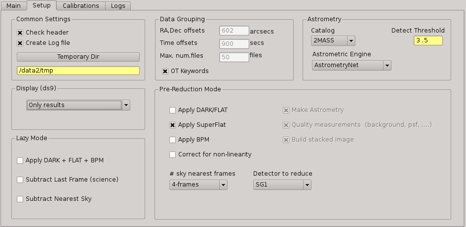
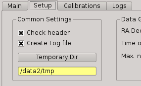
2.5.12.1. Common Settings
In this group you can set the next parameters:
Check header
Create log file
Temporary directory
2.5.12.2. Data grouping
It contains some parameters used for the data grouping when any OT keywords are present; in that case, PQL will try to group the files follwing the near in sky and time criterion:
RA,Dec offsets:
Time offsets:
Max. number of files:
If OT keywords are present, then check box ‘OT’ should be ckecked (default mode).
2.5.12.3. Astrometry
In this group you can set some parameters related with the astrometric calibration done during the processing:
Catalog: reference catalog used for the calibration (2MASS , USNO-B1, GSC 2.2, SDSS-R5)
Astrometric Engine: which tool you want to use to the astrometric calibration (SCAMP or Astrometry.net).
Detect threshold: the SExtractor threshold to be used to detect sources
2.5.12.4. Display
Here you can select which files are displayed automatically in the DS9. You have next options:
Only results (default): only FITS files created in the output directory as result of some processing
Only new files: only new FITS files detected in the input directory
All files: both new files detected in the input directory and the results in the output directry.
None: no files will be displayed
2.5.12.5. Lazy mode
Under this box, the user can select the operations to be executed when the Lazy Mode is activated in PQL. Currectly, the available and exclusive operations are:
Apply Dark + Flat + BPM
Subtract Last Frame (science)
Subtract Nearest Sky
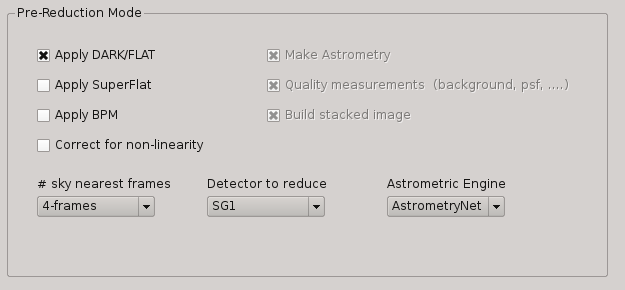
2.5.12.6. Pre-reduction
Under this box, the user can select the operations to be executed when the Pre-reduction Mode is activated in PQL. Currectly, the available and exclusive operations are:
Apply Dark and FlatField
Apply SuperFlat (default)
Apply BPM (Bad Pixel Map)
Correct for non-linearity
Select the number of frames to computer the sky bacground: 1-5 (default 4)
Detector to reduce: SG1 (default), SG2, SG3, SG4, SG123, All
2.5.13. Calibrations panel
This panel allows the user to set some of values for the search of master calibration files.

2.5.13.1. Set Calibs Dir
Pushing this button the user select the additional (external) directory from which the QL will look for master calibration files. Normally, it is used to provide to the QL with additional calibrations (dark, flat) from previous nights. Master calibrations found in the output directory will have higher priority than those ones.
This directory is also called ‘external calibration’ in PAPI command line:
-C EXT_CALIBRATION_DB, --ext_calibration_db=EXT_CALIBRATION_DB
                        External calibration directory (library of Dark & Flat
                        calibrations)
Or ext_calibration_db in the config file.
Then, if during the reduction of a ReductionSet(RS) no calibrations (dark, flat) are found in the current RS, then PAPI will look for them into this directory. If the directory does not exists, or no calibration are found, then no calibrations will be used for the data reduction. Note that the calibrations into the current RS have always higher priority than the ones in the external calibration directory.
2.5.13.2. Load last
When this button is pushed, the most recent master calibration files found in output directory and external calibrations are shown in the fields below.
If Use as default is click-checked, then the displayed files will be used as default calibrations when Apply Dark_FlatField_BPM is run. Otherwise, Apply Dark_FlatField_BPM routine will ask the user for the master calibration files to be used.
2.5.14. Log panel
It is an extension or duplicate of the Even Log window of the main panel, but with a wider area for messages.
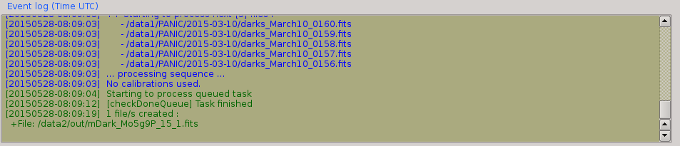
2.6. Event log window
The event log window shows important events and results generated by PQL. For example, the filename of the new files generated are shown, or the error produced while the processing of some sequence. This window is used only as output, and you cannot type any command on it.
2.7. Pop-up menu
It is a context pop-up menu that appears when the user select a file (or a set of them) in the Data List View and click the right mouse button. Next figure shows the options of that pop-up menu:
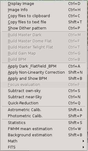
Some actions in the menu could be disabled and greyed out if they are not availabe or applicable to the selected files.
2.7.1. Display image
It displays the currect selected image in the SAOImage ds9 display; it will launch the ds9 application if it is not opened yet.
2.7.2. Image info
It is a quick way to see some basic information of the selected image. The information is mainly concerning the FITS structure and exposition times used. The information will be shown in the Event Log Window as follow:
---------------
SEF Filename : /data1/PANIC/2015-05-19_SS_zenith_Ks_1_3/SS_Ks_SG1_4_0024.fits
Image Shape : (32, 32)
Filter : Ks
ITIME : 0.045000
NCOADDS : 1
EXPTIME : 0.045000
TYPE : FOCUS
OT keywords : True
---------------
Of course, if you need any other information of the file, you can find it using the ‘ds9->File->Display Header…’ option.
2.7.3. Copy files to clipboard
It copies the current selected files to the clipboard. This way you could paste the full pathnames to any other file. It is quite useful when using the PAPI commands on the command line to run some operation that is not available on PQL.
2.7.4. Copy files to text file
If copies the current selected files into the specified text file. It is quite useful when using the PAPI command line to run some operation that is not available on PQL.
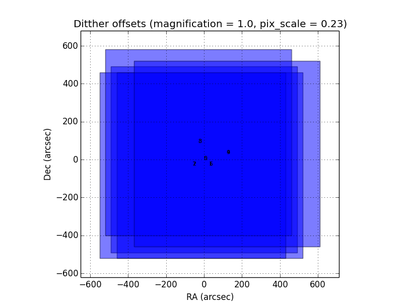
2.7.5. Show Dither pattern
It brings up a plot of the full FOV and with the dither offsets obtained from the RA,Dec coordinates found in the FITS header. You have to select a set of images in the Data List View and then right-button and Show Dither pattern.
2.7.6. Calibrations
Next options allow you to build the master calibration files from a given set of selected files.
2.7.6.1. Build Master Dark
This command is used to produce a master DARK file combining the set of files currectly selected in the Data List View. It checks that all the selected files are compliant, ie., have the same EXPTIME, NCOADD, ITIME, READMODE and shape. You only have to give the name of the master dark file to be created.
The master dark is computed using an average combine with a minmax rejection algorithm.
2.7.6.2. Build Master Dome Flat
This command is used to produce a Master DOME FLAT file combining the set of files currectly selected in the Data List View. It checks that all the selected files are compliant, ie., have the same FILTER, NCOADD, READMODE and shape. You have to select at least one DOME_FLAT_LAMP_OFF and one DOME_FLAT_LAMP_ON image, and then provide the name for the master dome flat to create.
The procedure to create the master dome flat is as follow:
Check the EXPTIME , TYPE(dome) and FILTER of each Flat frame
Separate lamp ON/OFF dome flats
Make the median combine + sigmaclip of Flat LAMP-OFF frames
Make the median combine + sigmaclip of Flat LAMP-ON frames
Subtract lampON-lampOFF (implicit dark subtraction)
(optionally) Normalize the flat-field with median (robust estimator)
Note that we do not need to subtract any MASTER_DARK; it is not required for DOME FLATS (it is done implicitly because both ON/OFF flats are taken with the same Exposition Time).
2.7.6.3. Build Master Twlight (sky) Flat
This command is used to produce a Master SKY FLAT file from a set of files currectly selected in the Data List View. It checks that all the selected files are compliant, ie., have the same FILTER, NCOADD, READMODE and shape. You have to select at least three SKY_FLAT images (dusk or dawn). The procedure will look for the required master dark frames to subtract in the current output directory and in the external calibration directory. If some of the master dark are not found, then the procedure will fail.
The procedure to create the master sky flat is as follow:
Check the TYPE (sky flat) and FILTER of each Flat frame If any frame on list missmatch the FILTER, then the master twflat will skip this frame and continue with then next ones. EXPTIME do not need be the same, so EXPTIME scaling with ‘mode’ will be done.
Check either over or under exposed frames ( [10000 < mean_level < 40000] ADUs )
We subtract a proper MASTER_DARK, it is required for TWILIGHT FLATS because they might have diff EXPTIMEs.
Make the combine (median + sigclip rejection) the dark subtracted Flat frames scaling by ‘mode’.
Normalize the sky-flat wrt SG1 detector, dividing by its mean value.
2.7.6.4. Build GainMap
This command is used to produce a Master GainMap file from a set of files currectly selected in the Data List View. It checks that all the selected files are compliant, ie., have the same FILTER, NCOADD, READMODE and shape. You have to select at least three flat frames (dome, dusk or dawn). For sky flats, the procedure will look for the required master dark frames to subtract in the current output directory and in the external calibration directory. If some of the master dark are not found, then the procedure will fail. Dome flat do not need dark subtraction.
The procedure to create the master sky flat is as follow:
Check the TYPE (sky flat) and FILTER of each Flat frame If any frame on list missmatch the FILTER, then the master twflat will skip this frame and continue with then next ones. EXPTIME do not need be the same, so EXPTIME scaling with ‘mode’ will be done.
Create the proper master dome/sky flat.
#. Once the master dome flat is created, the procedure will compute the gainmap as follow:
2.7.6.5. Build BPM
TBC
2.7.6.6. Apply Dark & FlatField & BPM
This option subtracts a master dark file, then divides by a flat field and finally mask the bad pixels on the current selected files. The master dark and master flatfield files can be searched for automatically into the output and external calibration directories or can be selected manually by the user.
If some of them (dark or flat) are not found or selected (pressing Cancel in the file dialog), then it will not be used or applied.
In the case of the bad pixel mask (BPM), it cannot be selected, but specified in the PAPI config file. However, the user will be asked for about which action to do with the bad pixel mask, whether set bad pixels as NaNs, fix bad pixels with an interpolation algorithm or do nothing with BPM.
2.7.6.7. Apply Non-Linearity Correction
It applies the Non-Linearity correction to the selected file (or set of files) in the Data List View and show the result in ds9; it also set bad pixels to NaN, and will be displayed as green pixels (or the default color configured in ds9->Edit->Preferences->General->Color) on the display.
The corrected image is saved in the output directory with a _LC suffix.
The master Non-Linearity correction file used for the correction is defined in the configuration file.
2.7.6.8. Apply and show BPM
This command can be used to apply the BPM to the selected file in Data List View the and show the results (NaNs) as green pixels (or the default color configured in ds9->Edit->Preferences->General->Color) on the display.
The bad pixel masked image is saved in the output directory with a _BPM suffix.
The master Bad Pixel Mask file used is defined in the configuration file.
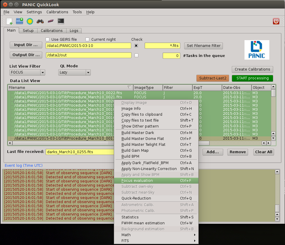
2.7.7. Focus evaluation
The Focus evaluation procedure is based in the IRAF starfocus routine. It only differs on the final plot that is obtained from non-saturated stars, and the best focus is computed computing the curve fit of these points. The PSF size is measured with the the FWHM of the best fit Moffat profile (MFWHM).
Once you have obtained a focus series using the Observation Tool, the procedure to evaluate and get the best focus value for that serie is as follow:
Warning
The input images of the focus series should be saved as SEF (Single Extension FITS), because IRAF starfocus does not works with MEF files. However, if your focus series was saved as SEF, the routine will previously convert to SEF, and then you should not have to do any other conversion.
Select the files of the focus series from the Data List View
Right-click and select Focus evaluation. An IRAF console and ds9 windows will bring up, and the first file of the focus series will be displayed on ds9.
Focus the mouse over the stars you think are nice for the evaluation and type m or g (give the profile of the selected star).

When you have finished of selecting all the stars you want for the focus evaluation, type q.
Then, an IRAF interactive graphics with the first fit will appear, and the best focus obtained. On that graphics, you should remove the images/stars/focus/points that you consider are not good for the focus evaluation (outliers); for this, type x and then i/s/f/p. Type u to undo the removing of the outliers. If you need more info about this commands see starfocus
Starfocus Cursor Commands:
When selecting objects with the image cursor the following commands are available.

?  Page cursor command summary
g  Measure object and graph the results.
m  Measure object.
q  Quit object marking and go to next image.
At the end of all images go to analysis of all measurements.

:show  Show current results.
When in the interactive graphics the following cursor commands are available. All plots may not be available depending on the number of focus values and the number of stars.

?  Page cursor command summary
a  Spatial plot at a single focus
b  Spatial plot of best focus values
d  Delete star nearest to cursor
e  Enclosed flux for stars at one focus and one star at all focus
f  Size and ellipticity vs focus for all data
i  Information about point nearest the cursor
m  Size and ellipticity vs relative magnitude at one focus
n  Normalize enclosed flux at x cursor position
o  Offset enclosed flux to by adjusting background
p  Radial profiles for stars at one focus and one star at all focus
q  Quit
r  Redraw
s  Toggle magnitude symbols in spatial plots
t  Size and ellipticity vs radius from field center at one focus
u  Undelete all deleted points
x  Delete nearest point, star, or focus (selected by query)
z  Zoom to a single measurement
<space> Step through different focus or stars in current plot type


:beta <val>     Beta parameter for Moffat fit
:level <val>    Level at which the size parameter is evaluated
:overplot <y|n> Overplot the profiles from the narrowest profile?
:radius <val>   Change profile radius
:show <file>    Page all information for the current set of objects
:size <type>    Size type (Radius|FWHM)
:scale <val>    Pixel scale for size values
:xcenter <val>  X field center for radius from field center plots
:ycenter <val>  Y field center for radius from field center plots

The profile radius may not exceed the initial value set by the task
parameter.
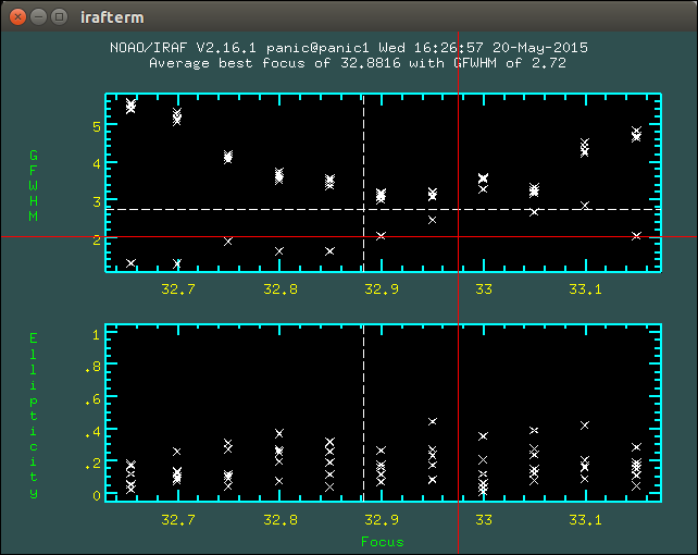
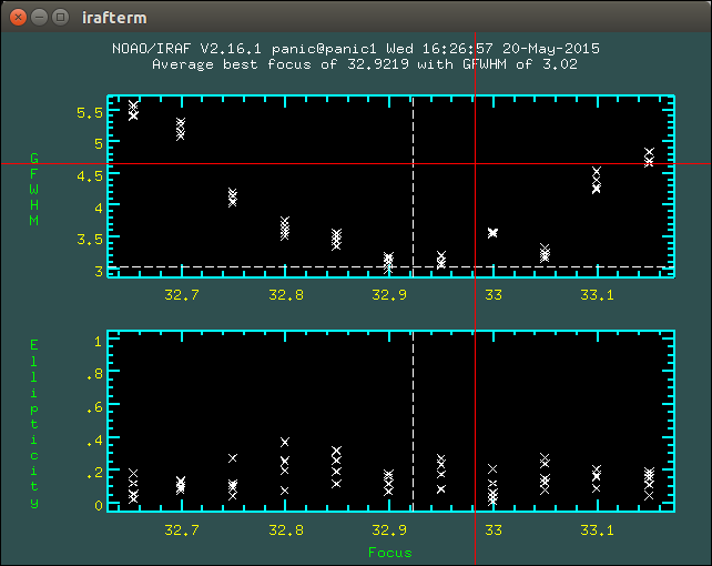
Once you have removed the outliers, type q (with the focus on the plot window) and you will get the final plot with the fit of the values, and the estimation for the best focus of the telescope.

Finally, the best focus obtained will be sent to the OT (which will ask you for confirmation) for setting the new telescope focus.
2.7.8. Subtract own-sky
It subtracts the background to the current selected image; the background computation is done using the own image. For this, -BACKGROUND option of SExtractor is used.
2.7.9. Subtract near-sky
It subtracts the background to the currect selected image using the closest (in time) images to the currectly selected. Once the close images have been found, PQL asks the user to confirm about them to proceede to the background computation and subtraction.
2.7.10. Quick reduction
It allows you to perform a quick reduction of the selected files (at least 5 files are required) on the Data List View.
If you only select one file, then the PQL will look for the nearest (in time) files and ask you to confirm about them and the desired name for the final coadd.
For the quick reducion, the pipeline will use the preferences set up on ‘Setup’ tab.
Once the quick reducion is done, the filename will be written in the Event Log Window, and if selected, it will be display on DS9 display.
2.7.11. Astrometric calibration
Note
Although the input FITS file does not need to be calibrared, it is recommended.
The astrometric calibration is built on top of Astrometry.net tool. The command asks you about which detector to use of the calibration (SG1/Q1, SG2/Q2, SG3/Q3 or SG4/Q4).
The new astrometrically calibrated file will be created in the output directory speficied earlier, and will have the same name as the original input file but ending with the .ast.fits suffix.
Once the astrometric calibration is done, you could look into the header keyword ROTANGLE, which gives you the rotation angle of the image. It can be useful to check whether the instrument rotator is set properly at the telescope.
2.7.12. Photometric calibration
Note
Your data is assumed to be calibrated. Dark subtraction, flat-fielding correction and any other necessary steps should have been performed before any data is fed to the photometric calibration.
We need to first distinguish between absolute and relative photometric calibration. Absolute photometric calibration would be required to determine the system throughput and/or the true magnitude of our stars. Relative photometry is a simpler task that would allow us to measure the uniformity and linearity of response across the detector. This section refers to absolute photometry.
The photometric calibration involves taking sufficiently long integrations with PANIC to get good a good SNR. The night must be photometric and the integration time and zenith angle need to be recorded. To reduce the dependence on zenith angle it would be best to take images within 30º of zenith. The photometric calibration can be performed using the saved images.
The photometric calibration will be useful for validating our throughput calculations. Using the photometric calibration to determine the true magnitudes of stars is more challenging.
2.7.13. Statistics
It gives some statistics (mean, mode, stddev, min, max) values of the currently selected image/s. If the image/s is/are MEF, then the command shows the stats of each extension [1-4], as shown in next example:
FILE                                                               MEAN     MODE       STDDEV   MIN     MAX
/data1/PANIC/2015-03-10/Standard_Star_FS27_March10_0060.fits[1]  6030.568  2377.875  8704.104  -1622.  49761.
/data1/PANIC/2015-03-10/Standard_Star_FS27_March10_0060.fits[2]  3069.276  3096.073  866.066  -5102.  54369.
/data1/PANIC/2015-03-10/Standard_Star_FS27_March10_0060.fits[3]  3852.473  3223.324  4300.289  -2509.  53549.
/data1/PANIC/2015-03-10/Standard_Star_FS27_March10_0060.fits[4]  3219.446  3060.269  2335.363  -4098.  53604.
/data1/PANIC/2015-03-10/Standard_Star_FS27_March10_0059.fits[1]  6059.874  2386.128  8698.008  -1629.  50722.
/data1/PANIC/2015-03-10/Standard_Star_FS27_March10_0059.fits[2]  3106.257  3151.27  849.268  -5109.  54257.
/data1/PANIC/2015-03-10/Standard_Star_FS27_March10_0059.fits[3]  3862.996  3222.919  4270.374  -2515.  53309.
/data1/PANIC/2015-03-10/Standard_Star_FS27_March10_0059.fits[4]  3258.566  3099.714  2331.496  -4100.  52753.
2.7.14. FWHM mean estimation
This command computes the FWHM of the selected image, using the FWHM_IMAGE value returned by SExtractor. For the computation, only stars which fulfill the next requirements are selected:
not near the edge of the detector
elliticiy < ellipmax (default = 0.3)
area > minare (default 32 pix)
snr > snr_min (default 5)
sextractor flag = 0 (the most restrictive!)
fwhm in range [0.1 - 20] (to avoid outliers)
For MEF files, the application will ask you which detector you want to use for the FWHM estimation.
Note
It is worth mentioning that SExtractor does a background subtraction when looking for objects and that the FWHM value is rather imperfect and overstimated compared with IRAF (imexam) values.
E. Bertin: “There are currently 2 ways to measure the FWHM of a source in SExtractor. Both are rather imperfect:
FWHM_IMAGE derives the FWHM from the isophotal area of the object at half maximum.
FLUX_RADIUS estimates the radius of the circle centered on the barycenter that encloses about half of the total flux. For a Gaussian profile, this is equal to 1/2 FWHM. But with most images on astronomical images it will be slightly higher.
A profile-fitting option will be available in the next version of SExtractor. I am currently working on it.”
2.7.15. Background estimation
This command shows the background image of the currently selected image, using the SExtractor feature ‘CHECKIMAGE_TYPE=BACKGROUND’.
2.7.16. Math operations
This option allows the next basic operations with the FITS files selected on the Data List View:
Sum images: it allows the selection of two or more images; single arithmetic sum will be done.
Subtract images: only two images can be selected.
Divide images: only two images can be selected.
Combine images (median + sigmaclip): it allows the selection of two or more images.
If FITS files are cubes (with the same dimension), then the math operation will be done plane by plane.
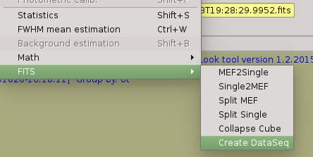
2.7.17. FITS operations
This option allows the next conversion operations with the FITS files selected on the Data List View:
MEF2Single: converts a MEF file to SEF file
Single2MEF: converts a SEF file to MEF file
Split MEF: extracts the extension (one per each detector) of the MEF file to individual files
Split Single: extracts the extension (one per each detector) of the SEF file to individual files
Collapse Cube: sums arithmeticly the planes of the given cube single plane 2D-image
Create DataSeq: modifies headers of the set of selected FITS files to create a new Data Sequece compliant with PAPI as they would be observed with the OT. This command can be usefil to fix or re-order broken sequences (observation was interrupted) or to remove or add files to a observed sequence. You will be asked for the type of sequence (DARK, DOME_FLAT, SKY_FLAT, FOCUS or SCIENCE) you want to create.
2.8. How do I …?
2.8.1. How to determine the telescope focus ?
To determine the telescope focus, you should run a OT focus serie around the guest value and then run the Focus Evaluation.
2.8.2. How to determine the field rotation ?
To determine the field rotation, firstly you should observe a enough crowded field and then run the astrometric calibration on it for each detector. Once you have the new FITS astrometrically calibrated, you have to look for the ROTANGLE keyword in the new header. For example:
ROTANGLE= -0.032836 / degrees E of N
2.8.3. How to inspect the profile of the stars in an image ?
You should follow the next steps:
select in the Data List View the image to inspect.
double-click to display the image into ds9 and zoom to the area you wish to inspect
go to the tool bar (or Tool menu) and open an IRAF console
type in the iraf console ‘imexam’
focus the mouse cursor on the ds9 display and type the imexam comand you wish for the inspection. For example, type *r* to show the radial profile of the selected star
once you have finished the inspection, type q to exit from imexam
2.8.4. How do I quick-reduce an observed sequence ?
There are two options:
if you know the files that compose the sequence, you can select them and then right-click and run the Quick-Reduction command.
go to the List View Filter and select GROUP; then look for the sequence you are looking for in the Data List View, right-click and select Reduce Sequece command.
For the quick reducion, the pipeline will use the preferences established on ‘Setup’ tab.
2.8.5. How do I quick-reduce an observed sequence using dark and flat master calibration files ?
You should follow the next steps:
1. Check your sequences are right,ie., they are well-formed and there were no interruption. It some sequece (calibration or science) is not well-formed, the you should use ‘FITS->Create DataSeq’ menu option in order to fix not well-formed sequence.
Create the output directory for the calibrations; then create the calibration pushing ‘Create calibrations’ button in the main panel.
3. When ‘Create calibrations’ have finished, go to ‘Calibration’ tab and select the directory having the master calibrations created just in setep #2.
4. Go to the ‘Setup->Pre-reduction Mode’ tab and check the option ‘Dark/Flat’ and select the detectors you want to process (SG1-SG4).
5. Finally, select the sequence you want to reduce, either selecting one by one the files in the Data List View or selecting the sequence with the ‘Group’ classification; then run ‘Quick-reduction’ from the Pop-up menu.
2.8.6. How do I make mosaics with PQL?
By default, PQL proccess or pre-reduce only the SG1 detector (Q1), and then no mosaic is built. However, you can go to the Setup Tab and modify in the Detector to reduce combo box the detector/s to reduce; in case of selecting All or SG123 (all less SG4), the corresponding mosaic will be generated.
Currently, PAPI aligns and coadds (using SWARP or Montage, see mosaic_engine in config file) the images as they are located on the sky to build the mosaic.
2.8.7. How do I make use of parallelisation ?
Just be sure the number of parallel parameter is set to True on the $PAPI_CONFIG file. When parallel=True, the pipeline will reduce each detector in parallel using all the cores available in your computer.
2.8.8. How do I report a issue ?
Please submit issues with the issue tracker on github.